The highs and lows of climate
Many factors contribute to the climatology of a given location, including how close to the equator you are, proximity to the ocean, and elevation. But when it comes to what causes climate to vary over seemingly short distances, few things can compare to the influence of topography.
Take my city, for example. I live in Asheville, in western North Carolina, a small city in the heart of the Southern Appalachians. I can drive ten minutes and be in one of the driest locations east of the Mississippi, or drive an hour and be in one of the wettest. That the temperature and precipitation patterns that we experience here can be so different from somewhere just a few miles away is due not just to elevation changes, but also the orientation of nearby mountains.
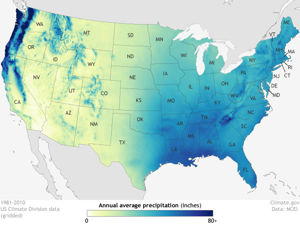
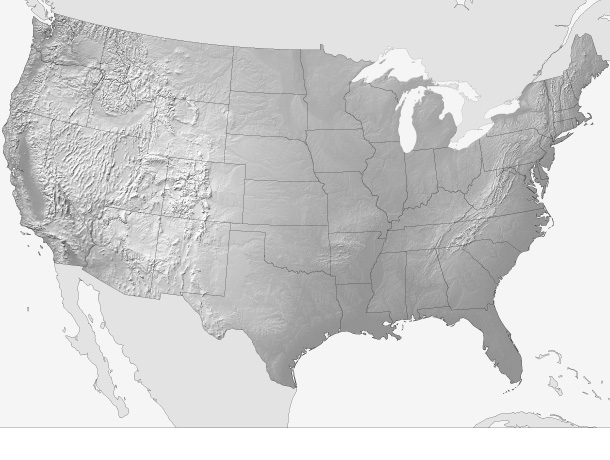
The influence of topography on climate shows up clearly in maps of annual average U.S. precipitation (1981-2010). The location of mountains and valleys are traced out by locally high precipitation amounts. Precipitation based on NOAA's nclimgrid data. Topography based on Natural Earth data. Maps by NOAA Climate.gov.
These changes in weather over a short distance can make forecasting the day-to-date weather very difficult, but they also presents challenges when calculating climate variables for the region as a whole. If you are a policy maker trying to decide where to build a reservoir or an entrepreneur trying to locate a new winery, understanding how geography and topography affect the local climate should be an important part of the decision making processing.
This edition of Beyond the Data will explore how topography—which is more than just elevation— the climate of a few locations across the country. We will also take a closer look at how scientists take topography into account when analyzing the climate system.
Mountains as rain makers and rain takers
One of the most dramatic examples of how topography can impact precipitation patterns occurs in the Pacific Northwest. The Cascade Mountains run from north to south in western Washington and Oregon. The mountains create a barrier to air moving eastward off the Pacific Ocean.
When the moist, oceanic air encounters the mountains it begins to rise. The rising air cools as it moves up and over the mountains, and much of its moisture condenses, forming clouds and precipitation. As the air continues moving to the east, it plunges down the other side of the mountains, warms up, and dries out. This phenomenon causes areas on the west side of the mountains to be much wetter than areas on the east side. Meteorologists call this contrast the orographic effect.
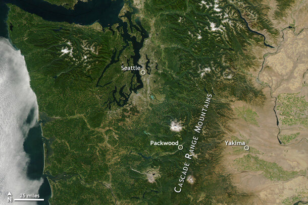
In the U.S., the Cascade Mountains are the king of orographic precipitation makers. The vegetation impacts—lush forests on the ocean-facing slopes, a browner, drier interior—are obvious in this NASA satellite image of Washington from September 11, 2002.
Let’s compare the precipitation climatology of Packwood and Yakima, both in Washington. Each location has similar elevation (~1060 feet) and latitude (~46.6°N), and they are only about 55 miles apart. But according to NOAA’s 1981-2010 climate normals, Packwood typically receives 56.0 inches of precipitation per year while Yakima receives just 8.3 inches! That’s because Packwood is located on the west side of the Cascade Mountains, while Yakima is on the east side.
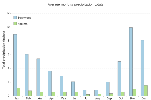
Monthly precipitation in Packwood (blue) and Yakima (green), based on U.S. Historical Climatology Network data from the National Centers for Environmental Information.
Brr! It’s cold up there!
Of course, mountains themselves can also directly impact a location’s climate. The higher the elevation of a place, the cooler its temperature tends to be. Here in western North Carolina, Asheville is located in a broad valley surrounded by high mountain peaks. The elevation of Asheville is about 2,240 feet above sea level. Twenty miles to the northeast, Mount Mitchell, at 6,684 feet above sea level, is the highest peak in the eastern United States.
The sharp elevation change over such a short distance means the average temperature for the two seemingly nearby locations is very different. The annual average temperature in Asheville is 56.5°F, while the annual average temperature on top of Mount Mitchell is 42.6°F (the weather station at Mount Mitchell has an elevation of 6,240 feet).
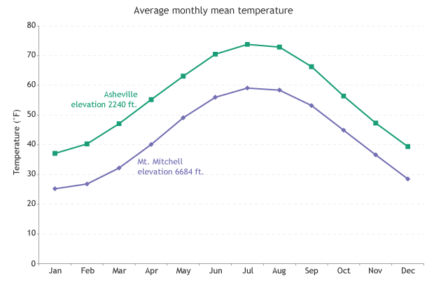
Monthly average temperatures in Asheville (green) and at Mt. Mitchell (purple) based on U.S. Historical Climatology Network data.
When calculating climate variables for an area, like we do in our climate division dataset, we must take into account these temperature and precipitation changes due to topography. We do this by two methods described below.
Gridding to fill in the blanks
For the U.S. climate division dataset – the basis for our statewide and national climatic values – data are gridded on a 5 kilometer (~3.1 mile) grid. Looking back at our example comparing the temperature at Asheville to Mount Mitchell, if we didn’t grid the data, we might only have two data points in the area.
The process of putting the data onto the grid utilizes our knowledge of how temperature and precipitation behave with elevation changes. Based on mathematical formulas we can determine best estimates of the temperature and precipitation between those two locations. For example, if we know that the temperature at Mount Mitchell is 30°F and it is 50°F in Asheville, the temperature halfway up the mountain will be 40°F. This provides a better spatial representation of weather and climate data across the region.
Anomalies instead of absolutes
Another way take into account changes in topography is by using anomalies. Anomalies are defined as the difference between a variable and a baseline, which is often the climate “normal”. For example, if the temperature for a location is 55°F today and the 1981-2010 normal value for the day is 49°F, the anomaly would be +6°F.
Temperature anomalies change less over a distance than the absolute temperature, regardless of topography. For example, a summer month for a climate division may be cooler than average, both at a nearby mountain peak and in the valley below, even though the absolute temperatures may be quite different at the two locations.
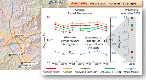
Average annual temperatures for four locations around Asheville, N.C. (top cluster of lines) from 2002-2008 are warmer than those at Mt. Mitchell (lower, blue line). Their absolute temperatures are all different, but their annual anomalies (blow-up at right) are nearly identical. Image by NCEI.
We then aggregate the anomalies over a spatial area to get a better representation of the climate conditions for a region and then use a baseline value, like the 1981-2010 normals, to get the absolute values for a the entire climate division. This strong relationship between relative temperatures from place to place becomes even stronger when we average over months and seasons: it is exceedingly rare for a high-elevation location to have a cold month while a neighboring low-elevation has a warm month, and vice versa.
So, where should your reservoir go?
Understanding how topography impacts local climate helps people make more informed decisions. Thinking back to the example of the water storage reservoir and winery location, would you want these investments located on the side of the mountain that faces the prevailing wind or on the drier side of the mountain? How about in a valley or on top of a mountain?
Climate scientists spend a great deal of effort to understand how the climate is changing and how modes of climate variability like El Nino will impact future temperature and precipitation. But before we take on those complex phenomena, we must make sure we account for the way non-atmospheric features like topography affect local weather and climate.